(a):
Calculate the present worth.
(a):
Explanation of Solution
The recovery rate for year 1 (RR1) is 0.3333, year 2 (RR2) is 0.4445, year 3 (RR3) is 0.1481, and year 4 (rr4) is 0.0741. Time period is indicated by ‘n’ and MARR is indicated by ‘i’.
Depreciation (D) can be calculated using the following formula:
Substitute the respective value in Equation (1) to calculate the depreciation in year 1.
The first year’s depreciation is $2,666.
The taxable income (TI) can be calculated using the following formula:
Substitute the respective value in Equation (2) to calculate the taxable income in year 1.
The first year’s taxable income is $834.
Tax (T) can be calculated using the following formula:
Substitute the respective value in Equation (3) to calculate the tax in year 1.
The first year’s tax is $333.
The cash flow after tax (CFATI) can be calculated using the following formula:
Substitute the respective value in Equation (4) to calculate the cash flow after tax in year 1.
The first year’s cash flow after tax is $3,167.
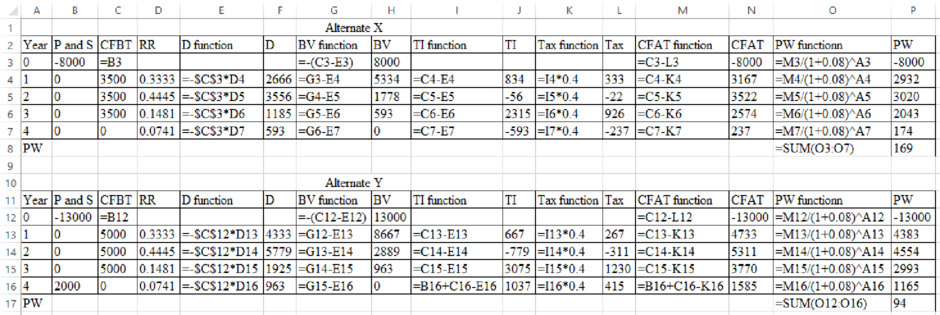
Table 1 shows the depreciation, taxable income, tax, and CFAT obtained using Equations (1), (2), (3) and (4).
Table 1
| Year | P | GI-OE | D | TI | T | CFAT |
| 0 | -8,000 | -8,000 | ||||
| 1 | 3,500 | 2,666 | 834 | 333 | 3,167 | |
| 2 | 3,500, | 3,556 | -56 | -22 | 3,522 | |
| 3 | 3,500 | 1,185 | 2,315 | 926 | 2,574 | |
| 4 | 0 | 0 | 593 | -593 | -237 | 237 |
The present worth (PW) can be calculated as follows:
The present worth of alternate X is $169.
Table 2 shows the depreciation, taxable income, tax, and CFAT of alternate Y obtained using Equations (1), (2), (3), and (4).
Table 2
| Year | P | GI-OE | D | TI | T | CFAT |
| 0 | -13,000 | -13,000 | ||||
| 1 | 5,000 | 4,333 | 667 | 267 | 4,733 | |
| 2 | 5,000 | 5,779 | -779 | -311 | 5,311 | |
| 3 | 5,000 | 1,925 | 3,075 | 1,230 | 3,770 | |
| 4 | 0 | 2,000 | 963 | 1,037 | 415 | 1,585 |
The present worth (PW) can be calculated as follows:
The present worth of project Y is $93. Since the present worth of project X is greater than project Y, select project X.
(a):
Calculate the time period.
(a):
Explanation of Solution
The present worth of alternate X and Y can be calculated using spreadsheet as follows:
Want to see more full solutions like this?
Chapter 17 Solutions
Engineering Economy


 Principles of Economics (12th Edition)EconomicsISBN:9780134078779Author:Karl E. Case, Ray C. Fair, Sharon E. OsterPublisher:PEARSON
 Engineering Economy (17th Edition)EconomicsISBN:9780134870069Author:William G. Sullivan, Elin M. Wicks, C. Patrick KoellingPublisher:PEARSON
 Principles of Economics (MindTap Course List)EconomicsISBN:9781305585126Author:N. Gregory MankiwPublisher:Cengage Learning
 Managerial Economics: A Problem Solving ApproachEconomicsISBN:9781337106665Author:Luke M. Froeb, Brian T. McCann, Michael R. Ward, Mike ShorPublisher:Cengage Learning
 Managerial Economics & Business Strategy (Mcgraw-...EconomicsISBN:9781259290619Author:Michael Baye, Jeff PrincePublisher:McGraw-Hill Education