
Videos
The article “Chemithermomechanical Pulp from Mixed High Density Hardwoods” (TAPPI, July 1988: 145–146) reports on a study in which the accompanying data was obtained to relate y = specific surface area (cm2/g) to x1 = % NaOH used as a pretreatment chemical and x2 = treatment time (min) for a batch of pulp.
| *1 | X2 | y |
| 3 | 30 | 5.95 |
| 3 | 60 | 5.60 |
| 3 | 90 | 5.44 |
| 9 | 30 | 6.22 |
| 9 | 60 | 5.85 |
| 9 | 90 | 5.61 |
| 15 | 30 | 8.36 |
| 15 | 60 | 7.30 |
| 15 | 90 | 6.43 |
The accompanying Minitab output resulted from a request to fit the model
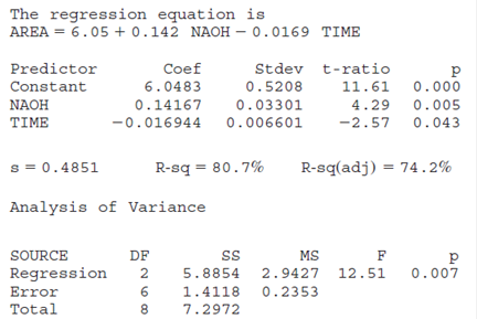
a. What proportion of observed variation in specific surface area can be explained by the model relationship?
b. Does the chosen model appear to specify a useful relationship between the dependent variable and the predictors?
c. Provided that % NaOH remains in the model, would you suggest that the predictor treatment time be eliminated?
d. Calculate a 95% CI for the expected change in specific surface area associated with an increase of 1% in NaOH when treatment time is held fixed.
e. Minitab reported that the estimated standard deviation

Trending nowThis is a popular solution!

Chapter 13 Solutions
Probability and Statistics for Engineering and the Sciences


- The depth of wetting of a soil is the depth to which water content will increase owing to extemal factors. The article "Discussion of Method for Evaluation of Depth of Wetting in Residential Areas" (J. Nelson, K. Chao, and D. Overton, Journal of Geotechnical and Geoenvironmental Engineering, 2011:293-296) discusses the relationship between depth of wetting beneath a structure and the age of the structure. The article presents measurements of depth of wetting, in meters, and the ages, in years, of 21 houses, as shown in the following table. Age Depth 7.6 4 4.6 6.1 9.1 3 4.3 7.3 5.2 10.4 15.5 5.8 10.7 4 5.5 6.1 10.7 10.4 4.6 7.0 6.1 14 16.8 10 9.1 8.8 Compute the least-squares line for predicting depth of wetting (y) from age (x). b. Identify a point with an unusually large x-value. Compute the least-squares line that results from deletion of this point. Identify another point which can be classified as an outlier. Compute the least-squares line that results from deletion of the outlier,…arrow_forwardFollowing are measurements of soil concentrations (in mg /kg) of chromium (Cr) and nickel (Ni) at20 sites in the area of Cleveland, Ohio. These data are taken from the article "Variation in NorthAmerican Regulatory Guidance for Heavy Metal Surface Soil Contamination at Commercial andIndustrial Sites" (A. Jennings and J. Ma, J. Environment Eng, 2007:587-609).Cr: 260 19 36 247 263 319 317 277 319 264 23 29 61 119 33 281 21 35 64 30Ni: 435 377 359 53 38 38 54 188 397 33 92 490 28 35 799 347 321 32 74 508 (d) Use these to construct comparative boxplots for the two sets of concentrations. (e) Using the boxplots, what differences can be seen between the two sets of concentrations?arrow_forwardA researcher is interested in testing the relationship between smoking and BMI (kg/m2) in adults aged 30-45. In order to test this association, the researcher divides smoking into currently more than a pack a day, currently less than a pack a day, and never smokers. The following table represents the BMIs for each participant enrolled by their respective smoking category. Current Smoker (≥1pack/day) Current Smoker (<1 pack/day Never Smoked 26.7 29.4 22.1 29.4 28.6 30.4 24.3 27.4 21.3 28.4 23.2 26.4 21.6 20.1 19.7 27.4 20.6 19.8 26.8 19.7 21.6 36.4 19.6 22.3 31.5 21.6 24.3 27.4 21.5 *Continue as though all assumptions for ANOVA are met. A) Calculate the MSW and MSB for the data represented above. B) Carry out a formal test for a one-way analysis of variance among the groups and interpret your results.arrow_forward
- The article “Snow Cover and TemperatureRelationships in North America and Eurasia” (J.Climate and Applied Meteorology, 1983: 460–469) usedstatistical techniques to relate the amount of snow coveron each continent to average continental temperature.Data presented there included the following ten observationson October snow cover for Eurasia during the years1970–1979 (in million km2):6.5 12.0 14.9 10.0 10.7 7.9 21.9 12.5 14.5 9.2What would you report as a representative, or typical,value of October snow cover for this period, and whatprompted your choice?arrow_forwardThe article “Wastewater Treatment Sludge as a Raw Material for the Production of Bacillus thuringiensis Based Biopesticides” (M. Tirado Montiel, R. Tyagi, and J. Valero, Water Research, 2001:3807–3816) presents measurements of total solids, in g/L, for seven sludge specimens. The results (rounded to the nearest gram) are 20, 5, 25, 43, 24, 21, and 32. Assume the distribution of total solids is approximately symmetric. a) Can you conclude that the mean concentration of total solids is greater than 14 g/L? Compute the appropriate test statistic and find the P-value. b) Can you conclude that the mean concentration of total solids is less than 30 g/L? Compute the appropriate test statistic and find the P-value. c) An environmental engineer claims that the mean concentration of total solids is equal to 18 g/L. Can you conclude that the claim is false?arrow_forwardThe article "Modeling Resilient Modulus and Temperature Correction for Saudi Roads" (H. Wahhab, I. Asi, and R. Ramadhan, Journal of Materials in Civil Engineering, 2001:298– 305) describes a study designed to predict the resilient modulus of pavement from physical properties. The following table presents data for the resilient modulus at 40°Cin10® kPa (y), the surface area of the aggregate in m²/kg (x1), and the softening point of the asphalt in °C (х). y X1 X2 1.48 5.77 60.5 1.70 7.45 74.2 2.03 8.14 67.6 2.86 8.73 70.0 2.43 7.12 64.6 3.06 6.89 65.3 2.44 8.64 66.2 1.29 6.58 64.1 3.53 9.10 68.6 1.04 8.06 58.8 1.88 5.93 63.2 1.90 8.17 62.1 1.76 9.84 68.9 2.82 7.17 72.2 1.00 7.78 54.1 The full quadratic model is y = + P,x, + PzX, + Pz*jXz + Pxx¡ + Bzx; + €. Which submodel of this full model do you believe is most appropriate? Justify your answer by fitting two or more models and comparing the results.arrow_forward
- 9.48) Acid gases must be removed from other refinery gases in chemical production facilities in order to minimize corrosion of the plants. Two methods for removing acid gases produced the corrosion rates (in mm/yr) are listed below in experimental tests: Method A: 0.3, 0.7, 0.5, 0.8, 0.9, 0.7, 0.8 Method B: 0.7, 0.8, 0.7, 0.6, 2.1, 0.6, 1.4, 2.3 Estimate the difference in mean corrosion rates for the two methods, using a confidence coefficient of 0.90. What assumptions must you make for your answer to be valid?arrow_forward5.25. Representative data on x = carbonation depth (in millimeters) and y = strength (in megapascals) for a sample of concrete core specimens taken from a particular building were read from a plot in the article “The Carbonation of Concrete Structures in the Tropical Environment of Singapore” (Magazine of Concrete Research [1996]: 293-300): Depth, x 8.0 20.0 20.0 30.0 35.0 40.0 50.0 55.0 65.0 Strength, y 22.8 17.1 21.1 16.1 13.4 12.4 11.4 9.7 6.8 a. Construct a scatterplot. Does the relationship between carbonation depth and strength appear to be linear? Yes, the relationship between carbonation depth and strength appears to be linear however it is a negative linear relation. b. Find the equation of the of the least-squares line.c. What would you predict for strength when carbonation depth is 25 mm?d. Explain why it would not be reasonable to use the least-squares line to predict strength when carbonation depth…arrow_forwardFifty male subjects drank a measured amount x (in ounces) of a medication and the concentration y (in percent) in their blood of the active ingredient was measured 30 minutes later. The sample data are summarized by the following information: n = 50 Ex = 112.5 Ex? = 356.25 %3D Ey = 4.83 Ey = 0.667 Exy = 15.255 0 < x < 4.5 Or= 0.875 Or= 0.709 Or= -0.846 Or=0.460 Or= 0.965arrow_forward
- The article "Electrical Impedance Variation with Water Saturation in Rock" (Q. Su, Q. Feng, and Z. Shang, Geophysics, 2000:68–75) reports measurements of permeabilities (in 10-3um?), porosities (in percent), and surface area per unit volume of pore space (in 104 cm -1) for several rock samples. The results are presented in the following table, denoting In Permeability by y, porosity by x1, and surface area per unit volume by x2. y -0.27 х, 19.83 X2 9.55 2.58 17.93 10.97 3.18 21.27 31.02 1.70 18.67 28.12 -1.17 7.98 52.35 -0.27 10.16 32.82 17.86 13.48 -0.53 57.66 -0.29 21.10 4.94 17.49 9.15 1.94 14.18 11.72 3.74 23.88 5.43 0.58 10.52 20.03 -0.56 18.92 13.10 -0.49 18.55 12.78 -0.01 13.72 40.28 -1.71 9.12 53.67 14.39 11.38 -0.12 26.75 -0.92 75.62 2.18 16.59 9.95 4.46 16.77 7.88 2.11 18.55 88.10 -0.04 18.02 10.95 Fit the model y = 6, + B,X1 + B>x2 + B3x;xX2 + ɛ. Compute the analysis of variance table. a. b. Fit the model y = Bo + B;X1 + B2X2 + ɛ. Compute the analysis of variance table. c.…arrow_forwardThe accompanying data set consists of observationson shower-flow rate (L/min) for a sample of n 5 129houses in Perth, Australia (“An Application of BayesMethodology to the Analysis of Diary Records in aWater Use Study,” J. Amer. Stat. Assoc., 1987:705–711):4.6 12.3 7.1 7.0 4.0 9.2 6.7 6.9 11.5 5.111.2 10.5 14.3 8.0 8.8 6.4 5.1 5.6 9.6 7.57.5 6.2 5.8 2.3 3.4 10.4 9.8 6.6 3.7 6.48.3 6.5 7.6 9.3 9.2 7.3 5.0 6.3 13.8 6.25.4 4.8 7.5 6.0 6.9 10.8 7.5 6.6 5.0 3.37.6 3.9 11.9 2.2 15.0 7.2 6.1 15.3 18.9 7.25.4 5.5 4.3 9.0 12.7 11.3 7.4 5.0 3.5 8.28.4 7.3 10.3 11.9 6.0 5.6 9.5 9.3 10.4 9.75.1 6.7 10.2 6.2 8.4 7.0 4.8 5.6 10.5 14.610.8 15.5 7.5 6.4 3.4 5.5 6.6 5.9 15.0 9.67.8 7.0 6.9 4.1 3.6 11.9 3.7 5.7 6.8 11.39.3 9.6 10.4 9.3 6.9 9.8 9.1 10.6 4.5 6.28.3 3.2 4.9 5.0 6.0 8.2 6.3 3.8 6.0 a. Construct a stem-and-leaf display of the data.b. What is a typical, or representative, flow rate?c. Does the display appear to be highly concentrated orspread out?d. Does the distribution of values appear to…arrow_forwardThe article “Arsenic and Mercury in Lake Whitefish and Burbot Near the Abandoned Giant Mine on Great Slave Lake” (P. Cott, B. Zajdlik, et al., Journal of Great Lakes Research, 2016:223–232) presents measurements of arsenic concentrations in fish found in Northern Canada. a) In a sample of 8 whitefish caught in Yellowknife Bay, the mean arsenic concentration in the liver was 0.32 mg/kg, with a standard deviation of 0.05 mg/kg. Find a 95% confidence interval for the concentration in whitefish found in Yellowknife Bay. b) In a sample of 8 whitefish caught in Baker Pond, the mean arsenic concentration in the liver was 0.55 mg/kg, with a standard deviation of 0.36 mg/kg. Should the Student’s t distribution be used to find a 95% confidence interval for the concentration in whitefish found in Baker Pond? If so, find the confidence interval. If not, explain why not.arrow_forward
 MATLAB: An Introduction with ApplicationsStatisticsISBN:9781119256830Author:Amos GilatPublisher:John Wiley & Sons Inc
 Probability and Statistics for Engineering and th...StatisticsISBN:9781305251809Author:Jay L. DevorePublisher:Cengage Learning
 Statistics for The Behavioral Sciences (MindTap C...StatisticsISBN:9781305504912Author:Frederick J Gravetter, Larry B. WallnauPublisher:Cengage Learning
 Elementary Statistics: Picturing the World (7th E...StatisticsISBN:9780134683416Author:Ron Larson, Betsy FarberPublisher:PEARSON
 The Basic Practice of StatisticsStatisticsISBN:9781319042578Author:David S. Moore, William I. Notz, Michael A. FlignerPublisher:W. H. Freeman
 Introduction to the Practice of StatisticsStatisticsISBN:9781319013387Author:David S. Moore, George P. McCabe, Bruce A. CraigPublisher:W. H. Freeman